Vehicle Detection and Tracking
Udacity Self Driving Car Nanodegree Project #5
Knowing where other cars are while driving is obviously extremely important. Modern multi-sensored self driving cars use their sensors largely to make predictions about their location and environment, including the other cars surrounding them. In this project, we will only focus on one type of sensor: a camera.
Histogram of Oriented Gradients (HOG)
Explain how (and identify where in your code) you extracted HOG features from the training images. Explain how you settled on your final choice of HOG parameters.
(Code for this section can be found in the “vehicle_detection_functions.py” file in lines 15-110, as well as the “Feature Extraction” Section section in the Jupyter notebook)
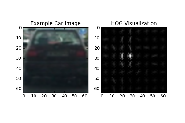
To extract Historgram of Oriented Gradient features (or HOG), I used the scikit-image function, hog(). The hog() function takes in a number of parameters, most of which I had to tune. Orientation was set to 9, which happens to be sufficient for the resolution of images we were dealing with. A higher bin size would have been better if we dealt with higher resolution images. I also had to specify the pixels per cell, as well as the cells per block. I specified 8 pixels per cell, and 2 cells per block. I selected these for the same reason I selected 9 bins, I felt it was sufficient for the resolution of images in our training data.
The color space used for this project is the YCrCb color space. The YCrCb color channel was chosen since it is a close alternative to RGB, and it gave better performance training my SVM (as well as having fewer false positives in my experiments). I decided to use all color channels of the YCrCb color space to get HOG features. This means that for each of the 3 color channels (Y, Cr, and Cb), I extracted separate HOG features and concatenated the results into a single vector.
The final feature vector included not only the HOG features of the 3 channels, but also the YCrCb color features (with 16 bins), and the spatial features of resized YCrCb images of size 32x32.
Concatenating all 3 of these feature representations results in a very long vector for each data image.
Describe how (and identify where in your code) you trained a classifier using your selected HOG features (and color features if you used them).
(Code for this section can be found in the “Data Prep” and “Linear SVC” Section section in the Jupyter notebook)
Our data was set up to be stored in a single numpy tensor, and then split up with the help of SciKit learns train_test_split function. Before using our image data, I first needed to convert every image in the data set into a new feature representation as described in the previous section. Using our new stretched out 8412 dimensional vector representation of our data, as well as their binary labels, we are almost ready to train a classifier.
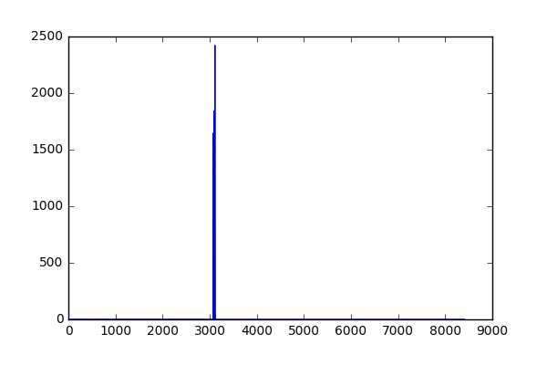
Before using our data, it is important to scale the features so that they are around the same scale, so that no specific feature (since we stacked 3 different representations together) will overpower the others. To alleviate this problem, I normalized all of the features using SciKit Learns preprocess tool called StandardScaler(). This ensures that we have zero mean and unit variance for the data in our training set. I fit the StandardScaler() to the training data, and transformed the training and test sets to the statistics of just the training data.
:
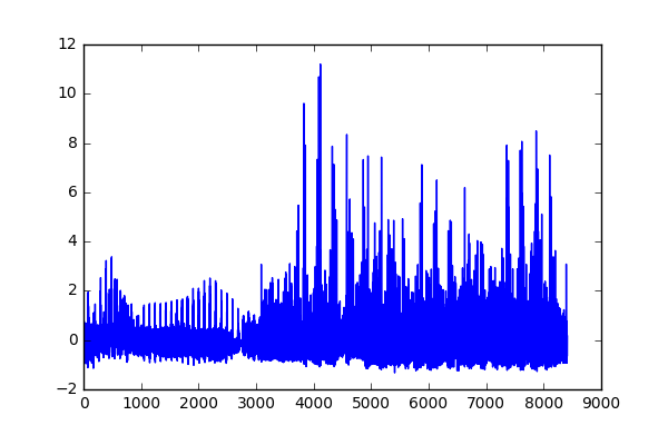
As you can see, there is a huge range of values that the combined 3 features can take (since the features themselves come from different types of representations). After scaling, that range is shrunk significantly, as well as now having zero mean and unit variance for cleaner training.
I decided to use a Linear SVM, as suggested in the lessons. This process was made simpler with the help of SciKit learns svm API. Specifically, I used the LinearSVC estimator.
My trained SVM was able to get 0.9901 accuracy on the test split.
Sliding Window Search
Describe how (and identify where in your code) you implemented a sliding window search. How did you decide what scales to search and how much to overlap windows?
(Code for this section can be found in the “vehicle_detection_functions.py” file in lines 236-313, as well as the “Test on road image” Section section in the Jupyter notebook)
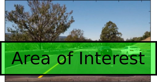
Rather than the conventional version of splitting our image into small windows, and having to do a full hog feature transformation on each window, I followed the advice in the lesson and did a HOG transform for the entire image (specifically, the portion of interest of the image). This cut down on compute time, and significantly sped up my pipeline.
After transforming an entire portion of an image to its hog representation, I then split that section up into chunks where we can just slice into (rather than HOG transform separately) the HOG features. I also do the cheap color and space feature transforms on those chunks. At each chunk, we stack the features up in the same order we stacked them prior to training, as well as preprocessing that new feature vector (with SciKit Learns StandardScalar() ) with the statistics we fit from the training data. We then make a prediction on whether or not there is a car in that chunk, and store that information into a “heat map”. Overlapping windows in which cars are predicted to be found, will have more “heat” associated with that specific area.
Instead of having different window sizes to search with, I scaled the entire image instead of the window. Keeping the window size the same, and adjusting the scale of the entire image, are very similar operations, and should result in similar (not exactly the same) results. That being said, I only used one scaling value (of 1.2) in my entire pipeline, which was sufficient to get reasonable results. I also specified a step size of 1 cell at a time for the overlap, which is equivalent to a 0.875 overlap with the window scheme (quite alot, but gave me reasonable results).
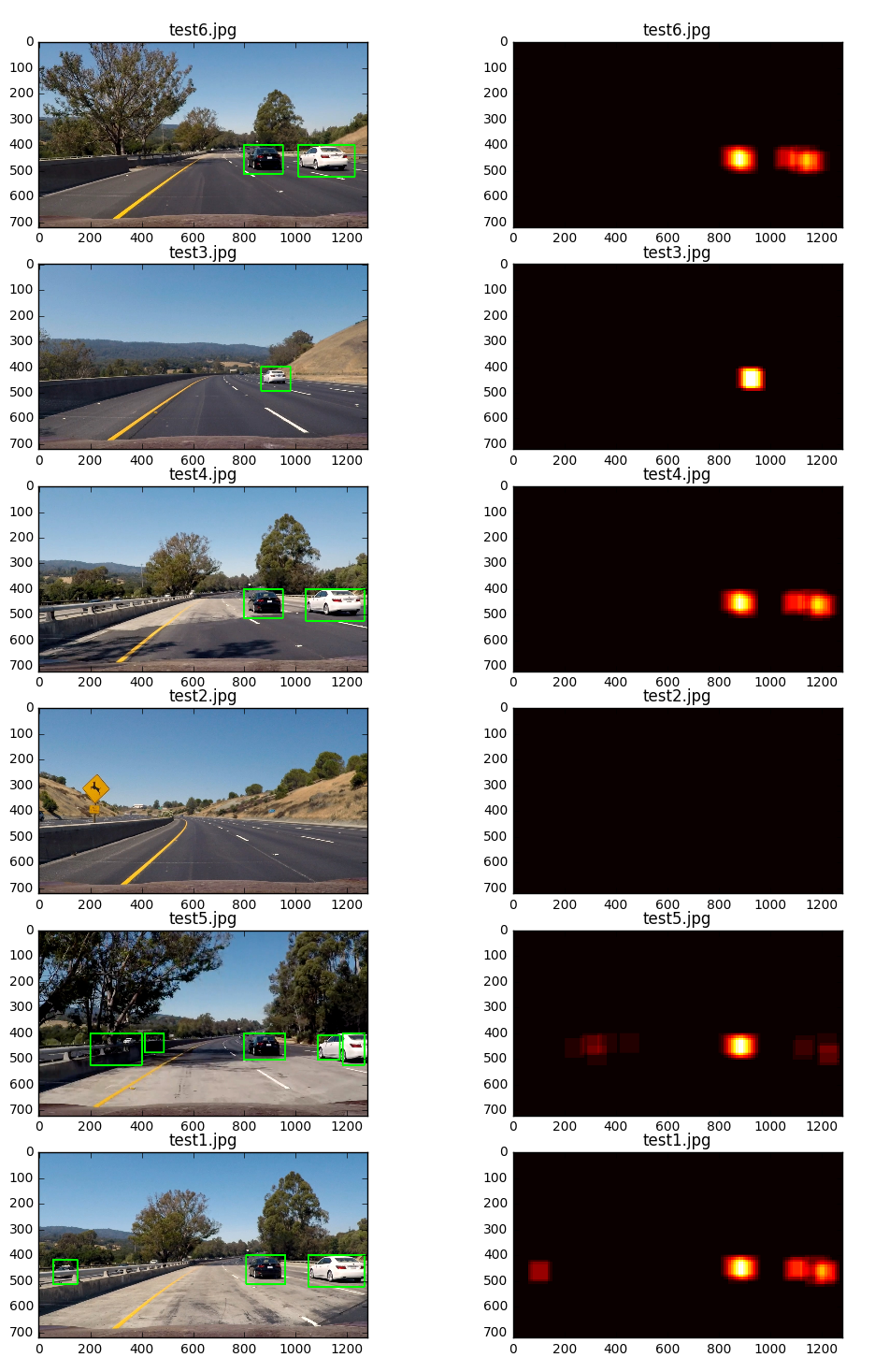
As you can see from the example above, there are a few false positives. It also picks up cars from the other side of the freeway (which is not necessarily useful information).
Show some examples of test images to demonstrate how your pipeline is working. How did you optimize the performance of your classifier?
(Code for this section can be found in the “vehicle_detection_functions.py” file in lines 166-222, as well as the “Test on road image” Section section in the Jupyter notebook)
(Examples of test images can be seen in the previous section)
In order to select my classifier, I tried out different combinations of color spaces and HOG parameters. The two parameters I found improved my classifier were the number of HOG channels, as well as the color channel used. I ended up choosing to use all HOG channels, as well as the YCbCr color space (over RGB).
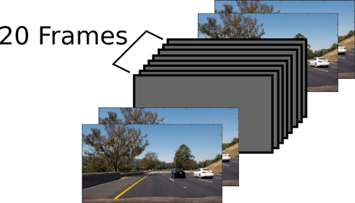
To improve on the reliability of the classifier, I leveraged the temporal structure provided by video (not present in single frames). By leveraging temporal information, we can aggregate predictions over a series of frames, and get a stronger classifier with less false positives.
To do so, I created a class to keep track of the heatmaps. This class is a very basic class which just holds a specified length (the length of time to recall) numpy array for a series of heatmaps. It also has functionality to aggregate the heat over N frames. Through trial and error, I found 20 frames of recall was sufficient enough to get me reasonable results.
Video Implementation
Provide a link to your final video output. Your pipeline should perform reasonably well on the entire project video (somewhat wobbly or unstable bounding boxes are ok as long as you are identifying the vehicles most of the time with minimal false positives.)
Describe how (and identify where in your code) you implemented some kind of filter for false positives and some method for combining overlapping bounding boxes.
(Code for this section can be found in the “vehicle_detection_functions.py” file in lines 178-198, as well as the “Test on road image” Section section in the Jupyter notebook)
(Much of this question is addressed in the 2nd part of the Sliding Window Search section of this writeup, but I will continue the discussion here)
With a large number of frames to aggregate, we are now more flexible with the heat threshold value we tune. I selected a very high heat threshold, 50 (through trial and error), since we had 20 frames of video to filter from. This significantly reduced the number of false positives, as well as reducing the number of cars detected on the other side of the freeway, since those cars are traveling in the opposite direction, they quickly leave the area of interest and are thus not providing consistent enough “heat” over the 20 frame period.
Here is the basic class used to keep track of the 20 heatmaps:
class Car_Heatmap():
	    def __init__(self, heatmap_frame, frames_to_recall):
			# Heatmap tensor from past N frames
			self.n_heatmaps = np.zeros((frames_to_recall,
					             heatmap_frame.shape[0],
					             heatmap_frame.shape[1]))

			# Heatmap combined from past N frames
			self.heatmap = np.sum(self.n_heatmaps, axis=0)

	    def update_heatmap(self):
			self.heatmap = np.sum(self.n_heatmaps, axis=0)
Discussion
Briefly discuss any problems / issues you faced in your implementation of this project. Where will your pipeline likely fail? What could you do to make it more robust?
At first, I struggled alot with the false positives popping up (briefly) at random times. So I decided to create the mentioned Car_Heatmap class to solve the problem.
My current implementation doesn’t pick up on cars close to the horizon, which might provide useful information. One way to fix this problem would be to add more scaled searches (equivalent to adding more windows of varying sizes), in order to pick up on the visually smaller cars in a camera view.
Some problems might occur when the car is moving at much higher speeds. If the driver is moving very fast compared to others on the road, the 20 frame period I hand selected may be too much time to aggregate results. That is, The “heat” of cars might not be sufficient enough to pass the high threshold (purposefully selected to be high due to the large number of frames to recall). Likewise, if other cars are moving very fast, the same problem might occur (similar to the cars on the other side of the lane). One way to solve this problem would be to further tune the number of frames to recall as well as the heat threshold.